A simple alternative search over Open Data Scotland’s dataset indexes

The Open Data Scotland website provides an up-to-date list of the Open Data resources about Scotland. It is being developed by the volunteer-run OD_BODS project team, and the idea for it originated from Ian Watt’s Scottish Open Data audit.

The website has been built using the JKAN framework which provides to end users, a ready-made search-the-datasets feature (try the search box near to the top of this page). However, its search can sometimes excessively exclude because it returns only those datasets whose metadata contain all of the search words, consecutively.

For instance, say that we wanted to find all datasets related to waste management. We might think of entering the search words: waste management recycl bin landfill dump tip. With JKAN, we would fairly much have to search for each of those words individually then collate the results.

Search tuning is its own whole field of research/area of business but, we have built a simple alternative to the JKAN search, to better support exploratory searching. Click on the image below to try the demo.

A animated GIF of an app to demo a simple alternative search over Open Data Scotland's dataset indexes

Stirling’s bin collection quantities per DataZone

A photograph by Lojze Jerala, of bins being emptied into a lorry in Ljubljana, Slovenia, 1959

This article is based on this programming notebook which provides more interactive detail.

đź‘‹ Introduction

Stirling council has published Open Data about its bin collections. Its data for 2021 includes town/area names. Our aim is to approximately map this data onto DataZones to extract insights.

DataZones are well defined geographic areas that are associated with (statistical) data, such as population data. This makes them useful when comparing between geographically anchored, per-person quantities – like Stirling’s bin collection quantities.

We have used the term approximately because mapping the bin collections data to DataZonesis not simple and unamibiguous. For example, the data may say that a certain weight of binned material was collected in “Aberfoyle, Drymen, Balmaha, Croftamie, Balfron & Fintry narrow access areas“, and this needs to be aportioned across several DataZones. In cases like this, we will aportion the weight across the DataZones, based on relative populations of those DataZones. Will the resulting approximation be accurate enough to be useful?

đź“Ť DataZones

Read the DataZones data from the Scottish government’s SPARQL endpoint

Each DataZone will have a name, a geographic boundary and a population.

Plot the DataZones on a map

đźš® Bin collections

Read the bin collections data from Stirling council’s Open Data website

🗂️ Map bin collection routes to DataZones

Apply a pipeline of data transformers/mappings to calculate the quantities per DataZone

📉 Plot the bin collection quantities per DataZone

Plot the monthly per-person quantities

Plot the monthly recycling percentages

🤔 Conclusions

The charts suggest that there are substantial differences between some DataZones, for example:

  • the per-person quantities chart indicates that there is roughly a Ă—3 difference between the best (Broomridge) and worst (Kippen and Fintry) DataZones,
  • and the recycling percentages chart indicates that there is roughly a Ă—2 difference between the best (City Centre) and worst (Bridge of Allan and University) DataZones.

Are these differences real? Well, they are too significant to have arisen due to a few bad data points or mappings. Ok then, could the differences be due to systematic differences in the method used to categorise and measure bin collection quantities, between DataZones? That’s unlikely since many of the DataZones at both ends of the ranking share the same processing/measurement facility.

Most of the DataZones exhibit a step change in both charts around Aug'21Nov'21 where (the majority of) the monthly quantities collected decrease and the recycling percentages increase.This coincides with Stirling council’s change to a four-weekly bin collection for grey bins (general waste) and blue bins (plastics, cartons & cans), and its Recycle 4 Stirling campaign. It’s understandable that that specific change to bin collections increased recycling percentages, but it doesn’t explain the decrease in monthly quantities. Perhaps there was also a change in the method of measurement/accounting, or that households took more of their waste to landfill sites themselves(!), or was it (at least partly) caused by the change in season?

It is good that Stirling council have begun to publish this data as Open Data into the public domain. It will open future, data-backed possibilities as it grows in volume and (hopefully) increases in fidelity. So, Stirling council, please keep on publishing the data (but make it more DataZone-friendly!).

A presentation of our work on the Participatory Accounting of Social Impacts

A presentation of our work on the Participatory Accounting of Social Impacts (in Scotland) – PASI.

Click on the image below to open the presentation in your web browser, then use <, > or SPACE BAR to navigate through the slides (and s to see the speaker notes).

DCS PASI presentation title page screenshot

Data flow in the proof-of-concept implementation for PASI

We have been exploring the idea of building a platform for the Participatory Accounting of Social Impacts (in Scotland) – PASI.  Waste reduction is the social impact that we are focussing on for our proof-of-concept (PoC) implementation, and the diagram (below) shows the flow of waste reduction related data, through our PoC.

A few notes about this PoC:

  • Potentially any individual/organisaton can be a “participant” (a peer-actor) in the PASI information system. A participant might publish data into PASI’s open, distributed (RDF) data graph; or/and consume data from it.
    In our PoC, participants can…
  • Supply measurement/observational data (quantities, times, descriptions). E.g. the instances of reuse/recycling supplied by ACE, STCMF, FRSHR and STCIL.
  • Provide reference metrics (measuring and categorisation standards). E.g. the carbon impact metric provided by ZWS.
  • Contribute secondary data (joining data, secondary calculations). E.g. the source→reference mappings, and the  calculated standardised waste reduction data contributed by DCS.
  • Build apps which consume the data from the PASI information system. E.g. a webapp which provides a dashboard onto waste reduction, for the general public.
  • Directly use the data in the distributed PASI graph. E.g. a federated SPARQL query constructed by a data analyst.

Data flow in the PASI PoC

Linked Open Data using a low-code, GraphQL based approach

“Might GraphQL be an easy means to query Linked Open Data?  Moreover, might it even be a handy means for building it?”

We use a product called JUXT Site, in exploring these questions.

JUXT Site

JUXT Site is a software product which offers a low-code approach for building HTTP-accessible databases. It has an add-on which allows for those databases (data models with their read & write operations) to be defined using GraphQL schemas.

JUXT Site is built on top of a database engine called XTDB which natively supports (temporal) graph queries (in the Datalog language). It has an add-on which supports (a subset of) SPARQL.

JUXT Site is Open-source software. It is in the pre-alpha phase of development (although its XTDB substrate is production ready).

So, JUXT Site’s has components which make it a promising platform on which to explore the questions at the head of this article. Here’s a diagram which summaries these components:

The relevant components of JUXT Site

(We made a small modification site-mod-sparql to JUXT Site, to surface XTDB’s SPARQL support.)

Next, we use JUXT Site’s GraphQL to build then query our linked data model.

Using GraphQL to build our linked data model

We took a subset of the linked data model that we defined for carbon savings and defined it using a GraphQL schema. The following snippets provide a flavour of that GraphQL definition.

Defining a record type

A StcmfRedistributedFood record says that a batch (weight batchKg) of food material was (time period from → to) redistributed to a destination. In our linked data model, further information about this – such as how the food material gets repurposed at the destination, and the lookup tables to calculate carbon savings – may be found by following links to other nodes in the data graph.

Here is how a StcmfRedistributedFood record type, is defined in GraphQL (on JUXT Site):

""" A batch of redistributed food material """
type StcmfRedistributedFood {

  id: ID!

  " The start of the period, inclusive "
  from: Date! @site(a: "pasi:pred/from") (1)

  " The end of the period, exclusive "
  to: Date! @site(a: "pasi:pred/to")

  " How the food material got used "
  destination: StcmfDestination
    @site( (2)
      q: { find: [e]
           where: [[e {keyword: "pasi:pred/type"} "StcmfDestination"]
                   [object {keyword: "pasi:pred/destination"} e]]
         }
    )

  " The weight in kilograms of this batch of food material "
  batchKg: Float! @site(a: "pasi:pred/batchKg")
}
  1. In GraphQL, a directive (@(…​)) can be used to say how a field should be mapped to/from to the underlying system.

    In JUXT Site, @site(…​) directives are used to map to/from structures in the underlying XTDB database. On this specific line, a: says that the field named from at the GraphQL level, should be mapped from the field named pasi:pred/from at the XTDB level.

    At the XTDB level, we use names like pasi:pred/from for our fields because such names are IRI-compliant, which means that they can be used as RDF predicates and queried using SPARQL.

  2. In this directive, we use the Datalog language to code how to find the appropriate StcmfDestination record in the underlying XTDB database.

Defining a query

Here is how a query operation to return all StcmfRedistributedFood records, is defined in GraphQL (on JUXT Site):

type Query {

  """ Return all records about batches of redistributed food material """
  stcmfRedistributedFood: [StcmfRedistributedFood]! (1)
}
  1. Simply declare that this returns a list ([…​]) of StcmfRedistributedFood records, and JUXT Site will take care of the implementation details.

Defining a mutation

Here is how a mutation operation to create or update a StcmfRedistributedFood record, is defined in GraphQL (on JUXT Site):

type Mutation {

  """ Create or update a record about a batch of redistributed food material """
  upsertStcmfRedistributedFood(

    id: ID
      @site(
        a: "xt/id"
        gen: {
          type: TEMPLATE
          template: "pasi:ent/StcmfRedistributedFood/{{from}}/{{to}}/{{destination}}" (1)
        }
      )

      " The start of the period, inclusive "
      from: Date! @site(a: "pasi:pred/from")

      " The end of the period, exclusive "
      to: Date! @site(a: "pasi:pred/to")

      " How the food material got used "
      destination: String! (2)
      destinationRef: ID
        @site(
          a: "pasi:pred/destination"
          gen: {
            type: TEMPLATE
            template: "pasi:ent/StcmfDestination/{{destination}}"
          }
        )

      " The weight in kilograms of this batch of food material "
      batchKg: Float! @site(a: "pasi:pred/batchKg")

  ): StcmfRedistributedFood @site(mutation: "update")
}
  1. We specify that a StcmfRedistributedFood record is identified by an IRI-compliant, natural key, composed from the from, to and destination values. Uniqueness is enforced over ID values therefore that combination of from, to and destination values will identity one or zero existing record(s).

  2. On invocation, this mutation will be supplied with a String value for the destination parameter. The destination String value is used to construct the ID of the targeted StcmfDestination record, and this ID is stored in a field named pasi:pred/destinationin the underlying XTDB database.

Querying our linked data model

We used JUXT Site’s GraphQL to build our linked data model (in terms of data structures and operations). Now let’s see what querying our data model looks like – firstly using GraphQL, then using SPARQL.

We will query not only for our StcmfRedistributedFood records but also for the associated information that we would need to create a waste reduction report which includes estimates of carbon savings. (Although we haven’t discussed this associated information in this article, showing the queries for it will make this exploration more informative.)

Querying using GraphQL

The query:

query PASI {
  stcmfRedistributedFood {
    batchKg
    from
    to
    destination {
      name
      refDataConnectors { (1)
        fraction
        refMaterial {
          carbonWeighting
          wasteStream
        }
        refProcess {
          name
        }
        enabler {
          name
        }
      }
    }
  }
}
  1. We haven’t discussed it in this article but we introduced an artificial direct connection, called refDataConnectors, into our data model to allow a query to walk easily to the reference data records that are needed to report on carbon savings.

The query’s raw result (truncated):

{
  "data": {
    "stcmfRedistributedFood": [
      {
        "batchKg": 87.61,
        "from": "2021-01-28",
        "to": "2021-01-29",
        "destination": {
          "name": "Used for human-food, bio-etc & sanctuary",
          "refDataConnectors": [
            {
              "fraction": 0.2,
              "refMaterial": {
                "carbonWeighting": "2.7",
                "wasteStream": "Mixed Food and Garden Waste (dry AD)"
              },
              "refProcess": {
                "name": "recycling"
              },
              "enabler": {
                "name": "Stirling Community Food"
              }
            },
            {
              "fraction": 0.8,
              "refMaterial": {
                "carbonWeighting": "4.35",
                "wasteStream": "Food and Drink Waste (wet AD)"
              },
              "refProcess": {
                "name": "reusing"
              },
              "enabler": {
                "name": "Stirling Community Food"
              }
            }
          ]
        }
      },
      {
        "batchKg": 0.48,
        "from": "2021-01-28",
        "to": "2021-01-29",
        "destination": {
          "name": "Used for compost-indiv",
          "refDataConnectors": [
            {
              "fraction": 1,
              "refMaterial": {
                "carbonWeighting": "3.48",
                "wasteStream": "Food and Drink Waste (Composting)"
              },
              "refProcess": {
[TRUNCATED]

The query’s result after formatting into a tabular report and calculating the carbonSaving column:

:enabler

:from

:to

:batchKg

:foodDestination

:ref_process

:ref_wasteStream

:ref_carbonSavingCo2eKg

Stirling Community Food

2021-01-28

2021-01-29

0.48

Used for compost-indiv

recycling

Food and Drink Waste (Composting)

1.67

Stirling Community Food

2021-01-28

2021-01-29

17.52

Used for human-food, bio-etc & sanctuary

recycling

Mixed Food and Garden Waste (dry AD)

47.31

Stirling Community Food

2021-01-28

2021-01-29

70.09

Used for human-food, bio-etc & sanctuary

reusing

Food and Drink Waste (wet AD)

304.88

Stirling Community Food

2021-01-29

2021-01-30

8.00

Used for compost-indiv

recycling

Food and Drink Waste (Composting)

27.84

Stirling Community Food

2021-01-29

2021-01-30

56.02

Used for human-food, bio-etc & sanctuary

recycling

Mixed Food and Garden Waste (dry AD)

151.26

Stirling Community Food

2021-01-29

2021-01-30

224.10

Used for human-food, bio-etc & sanctuary

reusing

Food and Drink Waste (wet AD)

974.82

Querying using SPARQL

SPARQL is used extensively by the Open Data community to query RDF datasets/graph databases.

Our chosen platform, JUXT Site (with XTDB), supports (a subset of) SPARQL. And we have defined our GraphQL-built data model to include RDF/SPARQL compliant names (i.e. IRI names for records and predicates/fields). So we can use SPARQL to query our data.

Here’s the SPARQL (almost) equivalent of the above GraphQL query:

PREFIX pasi: <pasi:pred/> (1)
SELECT ?enabler ?from ?to ?batchKg ?foodDestination ?ref_process ?ref_wasteStream ?ref_carbonSavingCo2eKg
WHERE {
  ?stcmfRedistributedFood pasi:type "StcmfRedistributedFood" ; (2)
                          pasi:from ?from ;
                          pasi:to ?to ;
                          pasi:batchKg ?origBatchKg ;
                          pasi:destination ?destination .
  ?destination pasi:name ?foodDestination .
  ?opsAceToRefData pasi:type "OpsStcmfToRefData" ; (2)
                   pasi:destination ?destination ;
                   pasi:fraction ?fraction ;
                   pasi:refMaterial/pasi:wasteStream ?ref_wasteStream ;
                   pasi:refMaterial/pasi:carbonWeighting ?carbonWeighting ;
                   pasi:refProcess/pasi:name ?ref_process ;
                   pasi:enabler/pasi:name ?enabler .
  BIND((?origBatchKg * ?fraction) AS ?batchKg) (3)
  BIND((?batchKg * ?carbonWeighting) AS ?ref_carbonSavingCo2eKg) (3)
}
ORDER BY ?enabler ?from ?to"
  1. We use pasi as the scheme part of all our IRIs. PASI is our an abbreviation for the (waste reduction) case study whose data model we’ve sampled in this article. It’s kind-of our root-level namespace.

  2. This SPARQL query uses two graph entry points StcmfRedistributedFood and OpsStcmfToRefData in order to walk to all the required graph nodes. Whereas, in GraphQL, we introduced an artificial direct connection, (refDataConnectors) which allowed the query to seamlessly walk to all the required graph nodes from a single graph entry point.

  3. The carbonSavings calculation is performed in SPARQL query. Whereas, with GraphQL, we performed the calculation outside of the query. Although, we could add an explicit carbonSavings field into data model with a GraphQL directive which specifies how to perform the calculation.

This SPARQL query can support the same tabular report as that supported by the GraphQL query, so we won’t bother (re)displaying that tabular report here.

Conclusions

  • JUXT Site offers an appealing low-code, GraphQL based approach for defining transactional, linked data systems. It’s a pre-alpha. Its sweet spot will probably be to back websites where humans drive query and transaction volumes.

  • With its ability to support RDF data models and SPARQL, it is a promising platform for Open Data. Currently, it supports only a subset of SPARQL but (again) it is only a pre-alpha.

  • So, “might GraphQL be an easy means to query Linked Open Data?“.

    Well, GraphQL was designed to describe the services that apps use. But, its query syntax is easier to understand that SPARQL’s (compare the above GraphQL and SPARQL queries) – so there is something to be said for providing a GraphQL interface as a means to explore an open dataset. With the proviso that GraphQL is more abstract/less exact than SPARQL, and it doesn’t directly support federated queries.

    They are, of course, different beasts. But a platform which is capable of supporting both over the same data might be a great way of servicing the audience for both.

  • Also – and we’ve not addressed these in this article but – the XTDB database (used by JUXT Site) has a number of other features that are important for transacting Linked Open Data: immutable records, temporal queries, and upcoming data-level authorisation scheme.

  • We see JUXT Site as a candidate platform on which to prototype our ‘PASI‘ system which will allow organisations to: upload their social impact data (including waste reduction data); validate it; assure security and track provenance; compose and accumulate it; and publish it as open linked data.

Using a literate programming tool to generate content

Literate programming tools weave data, code, visualisations and natural language into a flowing narrative. These tools are often used to construct tutorial-style documents that are based on tractable/generatable material.

For us, this sounded like a promising approach as a way to generate content since, one of our aims is to develop (website situated) how-to guides/tutorials based on the tractable waste datasets. So we created our first tutorial-style document using this approach: A walk-through on how to extract information from the data about business waste in Scotland. Here’s a screenshot of it:Screenshot of our first document generated using a literate programming tool

It uses:
Only minimal mark-up and programming code was required (see its source file), and it has proved to be a handy means to generate a data-based tutorial.

Annotating data points on our prototype website

On our requirements list is, to weave interest-based navigation maps through our data site. And feedback from the recent SODU 2021 conference, affirmed this:

I like the site’s tools and visualisations, but more needs to be done to help me navigate my path of interest through the prototype website.

In an exploratory step towards fulfilling that requirement, we have annotated some data points with explanations/narrative. The idea is that that these annotations could become waymarks in navigation maps, to guide users between the datapoints which underpin data-based stories. We might even imagine how clicking a ‘next’ button on a waymark would visually ‘fly’ the user to the next datapoint in the story (which is, perhaps, on a different graph or different page). But(!) back to our present, very simple proof-of-concept implementation…​

Here’s how the annotations look in our present, proof-of-concept implementation:

Annotations plotted on Inverclyde’s household waste generated graph

Each annotation is depicted by an emoji which is plotted beside a datapoint (on a graph, or in a table). When the user hovers over (or clicks on) an annotation’s emoji, a pop-up will display some informative text.

We want to code annotations just as we would any other dataset – as a straighforward CSV file. So we have built a data-drive annotation mechanism. This has allowed us to specify annotations, as data, in a CSV file like this:

Annotations specified in a CSV data file

Each annotation record contains datapoint coordinates which specify the datapoint against which the annotation is to be plotted. The datapoint coordinates include a record-type which specifies the dataset against which the annotation is to be plotted. (In this example, the specified dataset household-waste-derivation-generation is a derived dataset, based on the household-waste and population datasets.)

This proof-of-concept, data-driven, annotation mechanism has been useful because it has:

  1. given us a model with moving parts to learn from,

  2. provided hints about how annotations can be used to help users understand and navigate the data,

  3. shown us that we need more structure around the naming and storage of derived datasets (and their annotations), and

  4. uncovered the difficultlies of retro-fitting an annotations mechanism into our prototype-6 website. (Annotations are displayed using off-the-shelf Vega-lite tooltips and Bulma CSS dropdowns, but these don’t provide a satisfactory level of placement/control/interactivity. More customised webpage components will be needed to provide a better user experience.)

Building linked open data about carbon savings

linked open data for carbon savings

We have written a research report which walks through how we might build linked open data (LoD) about carbon savings from dissimilar data sources.

It outlines (using small samples from the datasets) how the data pipeline that feeds our prototype-6 webapp, works.

Building LoD about carbon savings - research report - coversheet